- Frequently we care about outcomes that have two values
- Alive/dead
- Win/loss
- Success/Failure
- etc
- Called binary, Bernoulli or 0/1 outcomes
- Collection of exchangeable binary outcomes for the same covariate data are called binomial outcomes.
Generalized linear models, binary data
Regression models
Brian Caffo, Jeff Leek and Roger Peng
Johns Hopkins Bloomberg School of Public Health
Key ideas
Example Baltimore Ravens win/loss
Ravens Data
download.file("https://dl.dropboxusercontent.com/u/7710864/data/ravensData.rda"
              , destfile="./data/ravensData.rda",method="curl")
load("./data/ravensData.rda")
head(ravensData)
  ravenWinNum ravenWin ravenScore opponentScore
1           1        W         24             9
2           1        W         38            35
3           1        W         28            13
4           1        W         34            31
5           1        W         44            13
6           0        L         23            24
Linear regression
\[ RW_i = b_0 + b_1 RS_i + e_i \]
\(RW_i\) - 1 if a Ravens win, 0 if not
\(RS_i\) - Number of points Ravens scored
\(b_0\) - probability of a Ravens win if they score 0 points
\(b_1\) - increase in probability of a Ravens win for each additional point
\(e_i\) - residual variation due
Linear regression in R
lmRavens <- lm(ravensData$ravenWinNum ~ ravensData$ravenScore)
summary(lmRavens)$coef
                      Estimate Std. Error t value Pr(>|t|)
(Intercept)             0.2850   0.256643   1.111  0.28135
ravensData$ravenScore   0.0159   0.009059   1.755  0.09625
Odds
Binary Outcome 0/1
\[RW_i\]
Probability (0,1)
\[\rm{Pr}(RW_i | RS_i, b_0, b_1 )\]
Odds \((0,\infty)\) \[\frac{\rm{Pr}(RW_i | RS_i, b_0, b_1 )}{1-\rm{Pr}(RW_i | RS_i, b_0, b_1)}\]
Log odds \((-\infty,\infty)\)
\[\log\left(\frac{\rm{Pr}(RW_i | RS_i, b_0, b_1 )}{1-\rm{Pr}(RW_i | RS_i, b_0, b_1)}\right)\]
Linear vs. logistic regression
Linear
\[ RW_i = b_0 + b_1 RS_i + e_i \]
or
\[ E[RW_i | RS_i, b_0, b_1] = b_0 + b_1 RS_i\]
Logistic
\[ \rm{Pr}(RW_i | RS_i, b_0, b_1) = \frac{\exp(b_0 + b_1 RS_i)}{1 + \exp(b_0 + b_1 RS_i)}\]
or
\[ \log\left(\frac{\rm{Pr}(RW_i | RS_i, b_0, b_1 )}{1-\rm{Pr}(RW_i | RS_i, b_0, b_1)}\right) = b_0 + b_1 RS_i \]
Interpreting Logistic Regression
\[ \log\left(\frac{\rm{Pr}(RW_i | RS_i, b_0, b_1 )}{1-\rm{Pr}(RW_i | RS_i, b_0, b_1)}\right) = b_0 + b_1 RS_i \]
\(b_0\) - Log odds of a Ravens win if they score zero points
\(b_1\) - Log odds ratio of win probability for each point scored (compared to zero points)
\(\exp(b_1)\) - Odds ratio of win probability for each point scored (compared to zero points)
Odds
- Imagine that you are playing a game where you flip a coin with success probability \(p\).
- If it comes up heads, you win \(X\). If it comes up tails, you lose \(Y\).
What should we set \(X\) and \(Y\) for the game to be fair?
\[E[earnings]= X p - Y (1 - p) = 0\]
Implies \[\frac{Y}{X} = \frac{p}{1 - p}\]
The odds can be said as "How much should you be willing to pay for a \(p\) probability of winning a dollar?"
- (If \(p > 0.5\) you have to pay more if you lose than you get if you win.)
- (If \(p < 0.5\) you have to pay less if you lose than you get if you win.)
Visualizing fitting logistic regression curves
x <- seq(-10, 10, length = 1000)
manipulate(
    plot(x, exp(beta0 + beta1 * x) / (1 + exp(beta0 + beta1 * x)),
         type = "l", lwd = 3, frame = FALSE),
    beta1 = slider(-2, 2, step = .1, initial = 2),
    beta0 = slider(-2, 2, step = .1, initial = 0)
    )
Ravens logistic regression
logRegRavens <- glm(ravensData$ravenWinNum ~ ravensData$ravenScore,family="binomial")
summary(logRegRavens)
Call:
glm(formula = ravensData$ravenWinNum ~ ravensData$ravenScore,
    family = "binomial")

Deviance Residuals:
   Min      1Q  Median      3Q     Max
-1.758  -1.100   0.530   0.806   1.495

Coefficients:
                      Estimate Std. Error z value Pr(>|z|)
(Intercept)            -1.6800     1.5541   -1.08     0.28
ravensData$ravenScore   0.1066     0.0667    1.60     0.11

(Dispersion parameter for binomial family taken to be 1)

    Null deviance: 24.435  on 19  degrees of freedom
Residual deviance: 20.895  on 18  degrees of freedom
AIC: 24.89

Number of Fisher Scoring iterations: 5
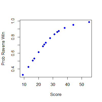
Ravens fitted values
plot(ravensData$ravenScore,logRegRavens$fitted,pch=19,col="blue",xlab="Score",ylab="Prob Ravens Win")

Odds ratios and confidence intervals
exp(logRegRavens$coeff)
          (Intercept) ravensData$ravenScore
               0.1864                1.1125
exp(confint(logRegRavens))
                         2.5 % 97.5 %
(Intercept)           0.005675  3.106
ravensData$ravenScore 0.996230  1.303
ANOVA for logistic regression
anova(logRegRavens,test="Chisq")
Analysis of Deviance Table

Model: binomial, link: logit

Response: ravensData$ravenWinNum

Terms added sequentially (first to last)

                      Df Deviance Resid. Df Resid. Dev Pr(>Chi)
NULL                                     19       24.4
ravensData$ravenScore  1     3.54        18       20.9     0.06 .
---
Signif. codes:  0 '***' 0.001 '**' 0.01 '*' 0.05 '.' 0.1 ' ' 1
Interpreting Odds Ratios
- Not probabilities
- Odds ratio of 1 = no difference in odds
- Log odds ratio of 0 = no difference in odds
- Odds ratio < 0.5 or > 2 commonly a "moderate effect"
- Relative risk \(\frac{\rm{Pr}(RW_i | RS_i = 10)}{\rm{Pr}(RW_i | RS_i = 0)}\) often easier to interpret, harder to estimate
- For small probabilities RR \(\approx\) OR but they are not the same!
Further resources
- Wikipedia on Logistic Regression
- Logistic regression and glms in R
- Brian Caffo's lecture notes on: Simpson's paradox, Case-control studies
- Open Intro Chapter on Logistic Regression